Abstract: We present a novel technique for direct visualization of unsteady flow on surfaces from computational fluid dynamics. The method generates dense representations of time-dependent vector fields with high spatio-temporal correlation using both Lagrangian- Eulerian Advection and Image Based Flow Visualization as its foundation. While the 3D vector fields are associated with arbitrary triangular surface meshes, the generation and advection of texture properties is confined to image space. Frame rates of up to 20 frames per second are realized by exploiting graphics card hardware. We apply this algorithm to unsteady flow on boundary surfaces of, large, complex meshes from computational fluid dynamics composed of more than 200,000 polygons, dynamic meshes with time-dependent geometry and topology, as well as medical data.

Full Length Video: 3:29 min, MPEG1 format (~44MB)
Paper: PDF format

Data Set	Visualization	File
(1) The data set is a piston cylinder and intake port. The piston head (not shown) defines the bottom of the surface mesh, varying with each crank angle. One half of a complete valve cycle is shown. In addition to analyzing the evolution of fluid flow from the intake port into the cylinder, this simulation data can also be used to analyze the formation of wall film -the term used to describe the liquid build-up on surfaces.
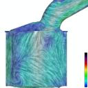
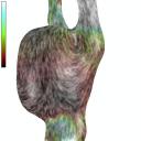
	(1.1) Higher spatial frequency textures are used. The amount of smearing and a color map indicate velocity magnitude.	900 frames (15.8MB)
	(1.2) Lower spatial frequency textures are used with a velocity clamp. The result visualization resembles LIC, and helps depict flow topology. A color map indicates velocity magnitude.	1200 frames (18.2MB)
	(1.3) Higher spatial frequency textures are used with a velocity mask. Smearing and a color map indicate velocity magnitude.	1000 frames (17.0MB)
	(1.4) This visualization demonstrates user-controlled spacial frequency of texture properties. i.e., multi-frequency Spot Noise. Smearing and a color map indicate velocity magnitude.	250 frames (5.7MB)
	(1.5) This visualization demonstrates user-controlled spacial frequency of texture properties. i.e., variable frequency LIC. A color map indicates velocity magnitude. Lower frequency textures may highlight topological features of the flow.	250 frames (5.2MB)
	(1.6) This one for those who are curious to see what the other side of the moving mesh looks like.	1100 frames (15.7MB)
(2) The data set is a cooling jacket. Visualization is very useful to observe the amounts of logitudinal and latitudinal flow. Stagnent flow is also very important here since this may represent areas of high temperature, causing fluid to boil.	(2.1) Higher spatial frequency textures are used with Spot Noise settings.	300 frames (8.5MB)
	(2.2) Lower spatial frequency textures with LIC settings. A velocity clamp facilitates the visualization of flow topology.	300 frames (5.5MB)
	(2.3) Here we apply a blue-yellow color map to the velocity magnitude. Yellow indicates areas of potential problems where stagnent fluid may heat up and cause boiling conditions.	300 frames (8.9MB)
	(2.4) We apply a blue-yellow color map to the velocity magnitude. Yellow indicates areas of potential problems where stagnent fluid may heat up and cause boiling conditions. User-controlled rotation is also used.	500 frames (12.1MB)
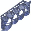
(3) The data set is two intake ports connected to a cylinder valve. It's a more complicated adaptive resolution surface consisting of 221,000 polygons. The views of user-controlled rotation are from the side, while the views of user-controlled zooming are from the top.	(3.1) We see the geometry rotating 270 degrees. Spot Noise settings with velocity color map.	500 frames (11.2MB)
	(3.2) We see the geometry rotating a full 360 degrees. Spot Noise settings with velocity color map.	650 frames (12.8MB)
	(3.3) user-controlled zooming with Spot Noise settings and velocity color map.	450 frames (11.8MB)
	(3.4) user-controlled zooming with Spot Noise settings, velocity color map, and velocity mask.	450 frames (12.2MB)
	(3.5) user-controlled zooming with LIC settings and velocity color map.	450 frames (9.6MB)
	(3.6) user-controlled zooming with LIC settings, velocity color map, and velocity mask.	450 frames (9.3MB)
	(3.7) user-controlled zooming extra close-up with a focus on 1 intake port -Spot Noise settings and velocity color map.	600 frames (17.7MB)
	(3.8) user-controlled zooming extra close-up with a focus on 1 intake port -Spot Noise settings, velocity color map, and velocity mask.	600 frames (15.6MB)
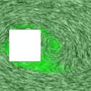
(4) This is a simulation of flow around a block often seen in flow visualization literature. As such, it can be used as a loose basis for comparison.	(4.1) Spot Noise, unsteady flow, close up	275 frames (7.0MB)
	(4.2) LIC, unsteady flow, a reverse velocity mask is used. That is, more opacity is used to highlight low velocity magnitude drawing the viewers attention to topological features of the flow.	400 frames (8.9MB)
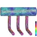
(5) This is a simulation of blood flow through the junction of 3 blood vessels. An abnormal pocket has formed at the junction, allowing stagnation of blood flow. Visualization also indicates the uneven distribution of blood flow to the outgoing vessles.	(5.1) An overview of the junction, with rotation, using a Spot Noise visualization. Smearing and hue indicate velocity magnitude.	500 frames (8.8MB)
	(5.2) An overview of the junction, with rotation, using an LIC visualization. Hue indicates velocity magnitude	500 frames (6.8MB)
	(5.3) A close-up view of the junction, with rotation, using a Spot Noise visualization. Texture smearing and hue indicates velocity magnitude	650 frames (14.7MB)
	(5.4) An close-up view of the junction, with rotation, using an LIC visualization. Hue indicates velocity magnitude	650 frames (10.1MB)
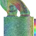
(6) Here we see unsteady fluid flow at the surface of an intake manifold. The ideal intake manifold distributes flow evenly to each piston valve. Visualization provides the engineer insight into this distribution.	(6.1) An overview of the intake manifold, using a Spot Noise visualization. Smearing and hue indicate velocity	1000 frames (22.7MB)
	(6.2) An overview of the intake manifold, using an LIC visualization. Hue indicates velocity magnitude	1000 frames (19.6MB)
	(6.3) Unsteady flow at the surface of an intake manifold using lower frequency LIC settings.	1000 frames (19.0MB)

This page is maintained by Robert S. Laramee.
In case of questions, please send email to: Laramee "at" VRVis.at.